Pandas怎样实现groupby分组统计
类似SQL:
select city,max(temperature) from city_weather group by city;
groupby:先对数据分组,然后在每个分组上应用聚合函数、转换函数
本次演示:
一、分组使用聚合函数做数据统计
二、遍历groupby的结果理解执行流程
三、实例分组探索天气数据
import pandas as pd
import numpy as np
# 加上这一句,能在jupyter notebook展示matplot图表
%matplotlib inline
df = pd.DataFrame({'A': ['foo', 'bar', 'foo', 'bar', 'foo', 'bar', 'foo', 'foo'],
                   'B': ['one', 'one', 'two', 'three', 'two', 'two', 'one', 'three'],
                   'C': np.random.randn(8),
                   'D': np.random.randn(8)})
df
|
A |
B |
C |
D |
| 0 |
foo |
one |
0.542903 |
0.788896 |
| 1 |
bar |
one |
-0.375789 |
-0.345869 |
| 2 |
foo |
two |
-0.903407 |
0.428031 |
| 3 |
bar |
three |
-1.564748 |
0.081163 |
| 4 |
foo |
two |
-1.093602 |
0.837348 |
| 5 |
bar |
two |
-0.202403 |
0.701301 |
| 6 |
foo |
one |
-0.665189 |
-1.505290 |
| 7 |
foo |
three |
-0.498339 |
0.534438 |
一、分组使用聚合函数做数据统计
1、单个列groupby,查询所有数据列的统计
df.groupby('A').sum()
|
C |
D |
| A |
|
|
| bar |
-2.142940 |
0.436595 |
| foo |
-2.617633 |
1.083423 |
我们看到:
1. groupby中的'A'变成了数据的索引列
2. 因为要统计sum,但B列不是数字,所以被自动忽略掉
2、多个列groupby,查询所有数据列的统计
df.groupby(['A','B']).mean()
|
|
C |
D |
| A |
B |
|
|
| bar |
one |
-0.375789 |
-0.345869 |
| three |
-1.564748 |
0.081163 |
| two |
-0.202403 |
0.701301 |
| foo |
one |
-0.061143 |
-0.358197 |
| three |
-0.498339 |
0.534438 |
| two |
-0.998504 |
0.632690 |
我们看到:('A','B')成对变成了二级索引
df.groupby(['A','B'], as_index=False).mean()
|
A |
B |
C |
D |
| 0 |
bar |
one |
-0.375789 |
-0.345869 |
| 1 |
bar |
three |
-1.564748 |
0.081163 |
| 2 |
bar |
two |
-0.202403 |
0.701301 |
| 3 |
foo |
one |
-0.061143 |
-0.358197 |
| 4 |
foo |
three |
-0.498339 |
0.534438 |
| 5 |
foo |
two |
-0.998504 |
0.632690 |
3、同时查看多种数据统计
df.groupby('A').agg([np.sum, np.mean, np.std])
|
C |
D |
|
sum |
mean |
std |
sum |
mean |
std |
| A |
|
|
|
|
|
|
| bar |
-2.142940 |
-0.714313 |
0.741583 |
0.436595 |
0.145532 |
0.526544 |
| foo |
-2.617633 |
-0.523527 |
0.637822 |
1.083423 |
0.216685 |
0.977686 |
我们看到:列变成了多级索引
4、查看单列的结果数据统计
# 方法1:预过滤,性能更好
df.groupby('A')['C'].agg([np.sum, np.mean, np.std])
|
sum |
mean |
std |
| A |
|
|
|
| bar |
-2.142940 |
-0.714313 |
0.741583 |
| foo |
-2.617633 |
-0.523527 |
0.637822 |
# 方法2
df.groupby('A').agg([np.sum, np.mean, np.std])['C']
|
sum |
mean |
std |
| A |
|
|
|
| bar |
-2.142940 |
-0.714313 |
0.741583 |
| foo |
-2.617633 |
-0.523527 |
0.637822 |
5、不同列使用不同的聚合函数
df.groupby('A').agg({"C":np.sum, "D":np.mean})
|
C |
D |
| A |
|
|
| bar |
-2.142940 |
0.145532 |
| foo |
-2.617633 |
0.216685 |
二、遍历groupby的结果理解执行流程
for循环可以直接遍历每个group
1、遍历单个列聚合的分组
g = df.groupby('A')
g
<pandas.core.groupby.generic.DataFrameGroupBy object at 0x00000123B250E548>
for name,group in g:
    print(name)
    print(group)
    print()
bar
     A      B         C         D
1  bar    one -0.375789 -0.345869
3  bar  three -1.564748  0.081163
5  bar    two -0.202403  0.701301

foo
     A      B         C         D
0  foo    one  0.542903  0.788896
2  foo    two -0.903407  0.428031
4  foo    two -1.093602  0.837348
6  foo    one -0.665189 -1.505290
7  foo  three -0.498339  0.534438
可以获取单个分组的数据
g.get_group('bar')
|
A |
B |
C |
D |
| 1 |
bar |
one |
-0.375789 |
-0.345869 |
| 3 |
bar |
three |
-1.564748 |
0.081163 |
| 5 |
bar |
two |
-0.202403 |
0.701301 |
2、遍历多个列聚合的分组
g = df.groupby(['A', 'B'])
for name,group in g:
    print(name)
    print(group)
    print()
('bar', 'one')
     A    B         C         D
1  bar  one -0.375789 -0.345869

('bar', 'three')
     A      B         C         D
3  bar  three -1.564748  0.081163

('bar', 'two')
     A    B         C         D
5  bar  two -0.202403  0.701301

('foo', 'one')
     A    B         C         D
0  foo  one  0.542903  0.788896
6  foo  one -0.665189 -1.505290

('foo', 'three')
     A      B         C         D
7  foo  three -0.498339  0.534438

('foo', 'two')
     A    B         C         D
2  foo  two -0.903407  0.428031
4  foo  two -1.093602  0.837348
可以看到,name是一个2个元素的tuple,代表不同的列
g.get_group(('foo', 'one'))
|
A |
B |
C |
D |
| 0 |
foo |
one |
0.542903 |
0.788896 |
| 6 |
foo |
one |
-0.665189 |
-1.505290 |
可以直接查询group后的某几列,生成Series或者子DataFrame
g['C']
<pandas.core.groupby.generic.SeriesGroupBy object at 0x00000123C33F64C8>
for name, group in g['C']:
    print(name)
    print(group)
    print(type(group))
    print()
('bar', 'one')
1   -0.375789
Name: C, dtype: float64
<class 'pandas.core.series.Series'>

('bar', 'three')
3   -1.564748
Name: C, dtype: float64
<class 'pandas.core.series.Series'>

('bar', 'two')
5   -0.202403
Name: C, dtype: float64
<class 'pandas.core.series.Series'>

('foo', 'one')
0    0.542903
6   -0.665189
Name: C, dtype: float64
<class 'pandas.core.series.Series'>

('foo', 'three')
7   -0.498339
Name: C, dtype: float64
<class 'pandas.core.series.Series'>

('foo', 'two')
2   -0.903407
4   -1.093602
Name: C, dtype: float64
<class 'pandas.core.series.Series'>
其实所有的聚合统计,都是在dataframe和series上进行的;
三、实例分组探索天气数据
fpath = "./datas/beijing_tianqi/beijing_tianqi_2018.csv"
df = pd.read_csv(fpath)
# 替换掉温度的后缀℃
df.loc[:, "bWendu"] = df["bWendu"].str.replace("℃", "").astype('int32')
df.loc[:, "yWendu"] = df["yWendu"].str.replace("℃", "").astype('int32')
df.head()
|
ymd |
bWendu |
yWendu |
tianqi |
fengxiang |
fengli |
aqi |
aqiInfo |
aqiLevel |
| 0 |
2018-01-01 |
3 |
-6 |
晴~多云 |
东北风 |
1-2级 |
59 |
良 |
2 |
| 1 |
2018-01-02 |
2 |
-5 |
阴~多云 |
东北风 |
1-2级 |
49 |
优 |
1 |
| 2 |
2018-01-03 |
2 |
-5 |
多云 |
北风 |
1-2级 |
28 |
优 |
1 |
| 3 |
2018-01-04 |
0 |
-8 |
阴 |
东北风 |
1-2级 |
28 |
优 |
1 |
| 4 |
2018-01-05 |
3 |
-6 |
多云~晴 |
西北风 |
1-2级 |
50 |
优 |
1 |
# 新增一列为月份
df['month'] = df['ymd'].str[:7]
df.head()
|
ymd |
bWendu |
yWendu |
tianqi |
fengxiang |
fengli |
aqi |
aqiInfo |
aqiLevel |
month |
| 0 |
2018-01-01 |
3 |
-6 |
晴~多云 |
东北风 |
1-2级 |
59 |
良 |
2 |
2018-01 |
| 1 |
2018-01-02 |
2 |
-5 |
阴~多云 |
东北风 |
1-2级 |
49 |
优 |
1 |
2018-01 |
| 2 |
2018-01-03 |
2 |
-5 |
多云 |
北风 |
1-2级 |
28 |
优 |
1 |
2018-01 |
| 3 |
2018-01-04 |
0 |
-8 |
阴 |
东北风 |
1-2级 |
28 |
优 |
1 |
2018-01 |
| 4 |
2018-01-05 |
3 |
-6 |
多云~晴 |
西北风 |
1-2级 |
50 |
优 |
1 |
2018-01 |
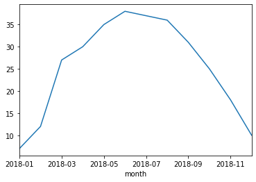
1、查看每个月的最高温度
data = df.groupby('month')['bWendu'].max()
data
month
2018-01     7
2018-02    12
2018-03    27
2018-04    30
2018-05    35
2018-06    38
2018-07    37
2018-08    36
2018-09    31
2018-10    25
2018-11    18
2018-12    10
Name: bWendu, dtype: int32
type(data)
pandas.core.series.Series
data.plot()
<matplotlib.axes._subplots.AxesSubplot at 0x123c344b308>
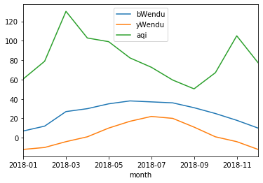
2、查看每个月的最高温度、最低温度、平均空气质量指数
df.head()
|
ymd |
bWendu |
yWendu |
tianqi |
fengxiang |
fengli |
aqi |
aqiInfo |
aqiLevel |
month |
| 0 |
2018-01-01 |
3 |
-6 |
晴~多云 |
东北风 |
1-2级 |
59 |
良 |
2 |
2018-01 |
| 1 |
2018-01-02 |
2 |
-5 |
阴~多云 |
东北风 |
1-2级 |
49 |
优 |
1 |
2018-01 |
| 2 |
2018-01-03 |
2 |
-5 |
多云 |
北风 |
1-2级 |
28 |
优 |
1 |
2018-01 |
| 3 |
2018-01-04 |
0 |
-8 |
阴 |
东北风 |
1-2级 |
28 |
优 |
1 |
2018-01 |
| 4 |
2018-01-05 |
3 |
-6 |
多云~晴 |
西北风 |
1-2级 |
50 |
优 |
1 |
2018-01 |
group_data = df.groupby('month').agg({"bWendu":np.max, "yWendu":np.min, "aqi":np.mean})
group_data
|
bWendu |
yWendu |
aqi |
| month |
|
|
|
| 2018-01 |
7 |
-12 |
60.677419 |
| 2018-02 |
12 |
-10 |
78.857143 |
| 2018-03 |
27 |
-4 |
130.322581 |
| 2018-04 |
30 |
1 |
102.866667 |
| 2018-05 |
35 |
10 |
99.064516 |
| 2018-06 |
38 |
17 |
82.300000 |
| 2018-07 |
37 |
22 |
72.677419 |
| 2018-08 |
36 |
20 |
59.516129 |
| 2018-09 |
31 |
11 |
50.433333 |
| 2018-10 |
25 |
1 |
67.096774 |
| 2018-11 |
18 |
-4 |
105.100000 |
| 2018-12 |
10 |
-12 |
77.354839 |
group_data.plot()
<matplotlib.axes._subplots.AxesSubplot at 0x123c5502d48>
相关推荐